Understanding the GPU memory Model
Your GPU has three kinds of memory -
Here's how H100 memory is laid out (and every other nvidia GPU):
1. Registers & Shared Memory
- Speed: "Lightning fast" (same clock as compute units)
- Capacity: Tiny (few KB per SM)
- Scope: Per streaming multiprocessor (SM)
- What lives here: Currently active data being computed on
CUDA enthusiasts might know shared memory as the place which you manage yourself and is shared among the threads in a block.
2. L2 Cache
- Speed: "Very fast"
- Capacity: ~50MB on H100
- Scope: Shared across the entire GPU
- What lives here: Behaves like how a cache works
3. HBM3 Global Memory
- Speed: "Much much slower" (as I initially put it)
- Capacity: 80GB on H100
- Scope: Everything
- What lives here: Model weights, activations, gradients
Again, CUDA enthusiasts will remember this place where we transfer the data before calling the kernel. It is the entry point of data in the GPU.
Actually this kind of hierarchy is nothing new. Even a simple CPU has the same concept. A fast SRAM which is called L1 cache, slightly slower SRAM called L2 cache and then your global RAM - DDR6, RD, SD, whatever based on which year you are looking at. The aim is to always increase the bandwidth. Send as much data as possible, as soon as possible to the processor.
But How Much Slower is "Much Much Slower"?
You can see that I have not quantified the speeds. I have used "Lightning Fast", "Very Fast" and "Much much slower"...
I looked up H100 specs and this is what I saw -
- Memory bandwidth: ~3,000 GB/s (3 × 10^12 bytes/second)
- Compute capability: ~1,000 TFLOPS (10^15 operations/second)
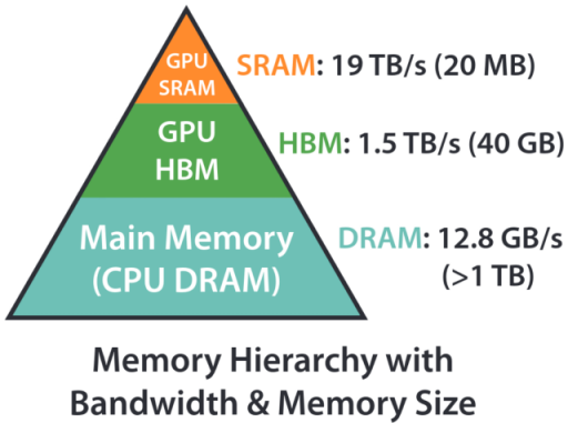
Memory Hierarchy in a typical GPU. Larger, slower memory in the bottom and faster, smaller memory in the top
Getting back to the Transformers Training aspect
Picture this: You're trying to train a transformer, and you're getting terrible GPU utilization. Your first instinct is probably the same as mine was - "throw more batch size at it!" But that led me to a crucial question:
Why does batch size matter for performance anyway?
That question sent me down a rabbit hole that will be the topic of my next few blog posts as I document my learnings. Let us recap the compute capability and memory bandwidth again -
- Memory bandwidth: ~3,000 GB/s (3 × 10^12 bytes/second)
- Compute capability: ~1,000 TFLOPS (10^15 operations/second)
What is this saying? Let us say you can add two numbers super fast. I give you (2, 6) and you return 8. You can process 5 tuples/second. To keep you busy all the time, I'll have to send atleast 5 tuples every second so that you have the data to go through. So the communication lanes between the memory and processor should be capable enough to send 5 tuples/second.
That is exactly what these numbers are trying to tell you. Compute Capability tells us how fast things are processed and Memory Bandwidth tells us how fast things are sent.
Operations per second: 10^15
Bytes per second: 3 × 10^12
Minimum FLOPs needed per byte: 10^15 / (3 × 10^12) = 333.33
So, to keep the GPU busy, we need to have 333.33 FLOPs per byte. Remember this number as this will serve as our North Start. If my operations don't achieve at least 333 FLOPs per byte of data transferred, my GPU compute units will be sitting idle for some part, waiting for data.
That's the threshold between being "memory-bound" vs "compute-bound." Super similar to IO-bound and compute-bound.
The Batch Size Revelation

Consider a simple matrix multiply: C = A x B where:
A:[batch_size, 4096, 4096]B:[4096, 4096](weights)C:[batch_size, 4096, 4096]
Let us do the FLOPs calculation first -
If we are multiplying a matrix of size m x k with another matrix of k x n, for each element, we will have k multiplications and k additions = 2k operations. It is actually k-1 additions but let us assume k. We will have m x n such elements and therefore, we will have 2 * k * m * n operations
FLOPs calculation: batch_size × 2 × 4096 × 4096 operations
Let us do the memory calculation next -
We have A that has batch_size * 4096 * 4096 elements. Let us assume FP16 data and therefore, each value is 16 bits or 2 bytes => batch_size * 4096 * 4096 * 2 bytes
Similarly, for B, we have 4096 * 4096 * 2 bytes
Memory transfer: (batch_size + 1) × 4096 × 4096 × 2 bytes (FP16)
Arithmetic intensity:
FLOPs/byte = (batch_size × 2 × 4096 x 4096) / ((batch_size + 1) × 4096 x 4096 × 2)
            = batch_size / (batch_size + 1)
For batch_size = 1: 0.5 FLOPs/byte For batch_size = 32: 0.97 FLOPs/byte For batch_size = ∞: 1.0 FLOPs/byte
LOL Even with infinite batch size, I'm getting 1 FLOP per byte, but I need 333 to saturate the compute! No wonder my training was slow.
But the real transformer network is super different
Transformer training isn't just isolated matrix multiplies. Between loading weights from HBM and being done with them, a lot happens:
Let us just take the MLP layer -
In an MLP layer:
intermediate = X @ W1(matrix multiply)intermediate = gelu(intermediate)(activation function)output = intermediate @ W2(another matrix multiply)
Each activation function operation adds FLOPs without requiring additional weight loading from slow HBM!
If we take a simple activation function like ReLU, it is checking if the value is greater than 0 and giving that. Otherwise giving a zero. That is a control instruction and it will be less than a FLOP but let us assume it is 1 FLOP. And this will happen for every element in the matrix. So, the number of FLOPs will be as many elements in the matrix.
Let me recalculate the FLOPs for a complete MLP layer:
But before we do, we need to define the dimensions. We will assume that we expand the layers in the hidden layer.
Typical MLP expansion layer. In our case the hidden layer has 4x more items than the input and the output again goes back to the same size.
[B, S, D] => [B, S, 4*D] => [B, S, D]
Memory transfers: (B×S×D + 8×DxD) × 2 bytes
FLOPs: 8×B×S×DxD + 4×B×S×D + 8xBxSxDxD operations
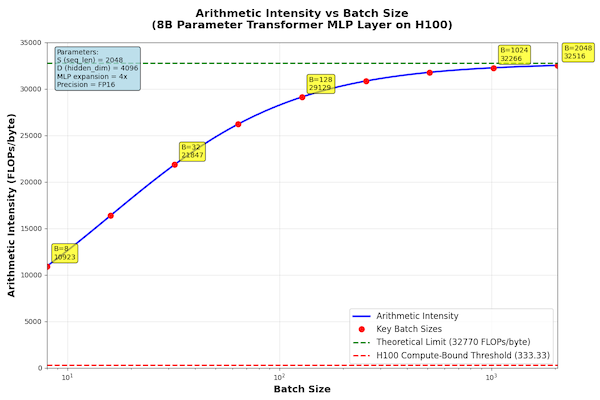
With B=32, S=2048, D=4096:
- Total FLOPs: 17,593,259,786,240
- Total bytes: 805,306,368
- Arithmetic intensity: 21,847 FLOPs/byte
This explains why MLP layers perform better than I expected!
So... Do we just keep increasing the batch size?
AI = 4×B×S×D×(4×D + 1) / [(B×S×D + 8×DxD) × 2]
As B becomes larger and larger, BxSxD dominates over 8xDxD and we can assume it is just O(BxSxD). And that B cancels out with the numerator.
In other words, as B increases, it is not factored into the calculation and AI starts plateuing...
With S=2048, I'm approaching ~2048 FLOPs/byte regardless of batch size. That's above our 333 threshold, but it means there's a point of diminishing returns for increasing batch size.
After a point, the arithmetic intensity starts plateauing
What this means in real life when using batch size
- Increasing Batch size is a proven way of improving performance - but it helps up to a point, then plateaus
- 333 FLOPs/byte is an important thing to understand
- Layer Design matters... specially a dense structure like MLP - operations between weight loads are "free" from point of view of memory
There are other GPU related issues that come into picture if we keep increasing batch size. One of the things is that if you have too large a batch size, matrix multiplications starts looking slow and that will eat into performance.
We will look into other constraints around increasing batch size in another post hopefully.